library("spiDE")

data(toySpiDE)
res <- spiDE(toySpiDE, condition = "condition", sigma = 30, index = "A", verbose = FALSE)
plotPatientSlopes(res, gene = c("G1", "G2"), index = "A", niche = "B")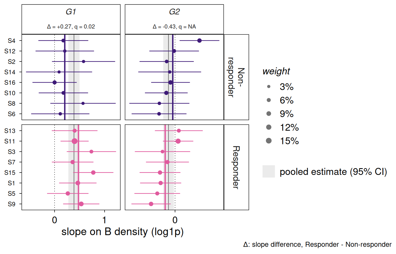
The evidence the tests weigh: every patient’s own slope of the gene’s expression in the index type on the niche type’s density (log1p), with an interval from its within-patient variance – the variance the tests use – and a point sized by the patient’s weight in them. The pooled estimate and its confidence interval are the grey band. With a condition the patients are split by it, each group’s weighted mean is a coloured line, and each strip gives the condition-specific slope difference and its q-value.
plotPatientSlopes(x, gene, index, niche, ci = 0.95)
x
|
a SpiDEResults from the slopes engine. |
gene
|
one or more genes, one column each. |
index, niche
|
the index and niche cell types. |
ci
|
the confidence level of the intervals. |
Read it for whether a call rests on patients that agree or on one or two heavily weighted ones, and for why a condition test is missing (each group needs three effective patients). Patients are ordered by group, then by their mean slope over the genes shown, so a row is one patient across genes.
a ggplot. p$data has one row per (gene, patient) with a slope: gene, patient, slope, se (within patient), weight (the patient’s share of the pooled test’s weights), condition and gene_lab (the strip label, plotmath). Change it like any ggplot, e.g. + theme(axis.text.y = element_blank()).
patientSlopes() for the numbers, plotNicheResponse() for the cells.
library("spiDE")
data(toySpiDE)
res <- spiDE(toySpiDE, condition = "condition", sigma = 30, index = "A", verbose = FALSE)
plotPatientSlopes(res, gene = c("G1", "G2"), index = "A", niche = "B")