library(spiDE)
library(SpatialExperiment)
data(toySpiDE)
toySpiDE
#> class: SpatialExperiment
#> dim: 20 2400
#> metadata(0):
#> assays(1): counts
#> rownames(20): G1 G2 ... G19 G20
#> rowData names(0):
#> colnames(2400): cell1 cell2 ... cell2399 cell2400
#> colData names(9): sample_id condition ... Area nCount
#> reducedDimNames(0):
#> mainExpName: NULL
#> altExpNames(0):
#> spatialCoords names(2) : x y
#> imgData names(0):
patients <- unique(as.data.frame(colData(toySpiDE))[, c("sample_id", "condition")])
table(patients$condition)
#>
#> Non-responder Responder
#> 8 8
table(toySpiDE$cell_type)
#>
#> A B C
#> 813 726 861spiDE
spiDE finds neighbourhood-dependent differential expression in spatial transcriptomics. Cells of one type do not behave the same everywhere in a tissue. A tumour cell sitting among fibroblasts may express a different set of genes from a tumour cell surrounded by other tumour cells, and the way it responds may differ between patients who respond to a treatment and patients who do not. spiDE asks, for a chosen index cell type, whether the expression of a gene changes with the local density of another cell type, which we call the niche, and whether that change differs between two conditions.
Doing this well is harder than it sounds. The cells of one patient share their genetics, their treatment and the way their sample was handled, and neighbouring cells share their local tissue environment. If every cell is treated as an independent observation, the more cells are measured the more certain a result looks, even when the patients disagree with each other. A condition such as response to treatment is a property of a patient, not of a cell, so the patient is the right unit of replication. spiDE builds this into every test: the evidence for a result is how consistently the niche slope behaves between patients, never how many cells were measured.
One hypothesis is one (gene, index type, niche type) combination, which we call a triplet. Each triplet gets up to two tests:
- The pooled test asks whether, within patients, the gene’s expression in the index type changes with the density of the niche type, consistently across patients.
- The condition-specific test asks whether that dependence differs between two conditions, such as responders and non-responders.
Both tests look at slopes within patients. A condition that only shifts a gene’s overall level, or only changes how much of a cell type patients have, is not tested here; those are questions for pseudobulk differential expression and composition analysis. The analysis runs in three steps, and each has its own function:
- Build the niches (
buildNiches()in R,build_niches()in Python) measures the density of every cell type around every cell. - Fit (
fitSpiDE()in R,fit_spide()in Python) fits a negative binomial regression for every gene in every index type, with a separate baseline for every patient, so that the niche coefficients are slopes within patients. - Test (
testSpiDE()in R,test_spide()in Python) tests those slopes across patients.
spiDE() in R and spide() in Python run all three in one call.
This website documents two packages that implement the same method: the R package spiDE and the Python package spidepy. Every step below is shown in both. Pick a language in any tab and all the tabs on the site follow. The example is the small simulated data set that ships with both packages, so nothing is subsampled or simplified to keep the page quick: the whole page runs in about a minute. The two packages are separate implementations of one method, so we should not expect identical output in general. On this data set the tables agree to numerical precision, which we check directly near the end of the page; on other data they agree qualitatively, with small numerical differences, and R vs Python lists where the two packages intentionally differ. The statistics are explained in The spiDE model, how well the tests hold up in Validation, and how many patients and cells a study needs in Designing a study.
Both packages can be installed as follows:
if (!requireNamespace("BiocManager", quietly = TRUE))
    install.packages("BiocManager")

BiocManager::install("BhuvaLab/spiDE")
spidepy is not on PyPI yet; install it from GitHub. The extra index gives a CPU-only build of PyTorch, which it needs through spanormpy:
pip install --extra-index-url https://download.pytorch.org/whl/cpu "spidepy @ git+https://github.com/BhuvaLab/spidepy.git"Load the data
We begin by loading a small simulated data set that ships with the package. It holds 16 patients, eight responders and eight non-responders, with 150 cells each, three cell types (A, B and C) and 20 genes. We planted exactly one effect in it: gene G1 is up-regulated in index type A, in responders only, in proportion to the local density of niche type B. Because we know the answer, we can check that spiDE finds it. The Python package ships the same data.
import spidepy as sp

adata = sp.datasets.toy_spide()
print(adata)
#> AnnData object with n_obs × n_vars = 2400 × 20
#>     obs: 'sample_id', 'condition', 'x', 'y', 'cell_type', 'Age', 'cell_id', 'Area', 'nCount'
#>     uns: 'r_call', 'r_dim'
#>     obsm: 'spatial'
#>     layers: 'counts', None (.X)
patients = adata.obs[["sample_id", "condition"]].drop_duplicates()
print(patients["condition"].value_counts())
#> condition
#> Responder        8
#> Non-responder    8
#> Name: count, dtype: int64
print(adata.obs["cell_type"].value_counts())
#> cell_type
#> C    861
#> A    813
#> B    726
#> Name: count, dtype: int64
The same 2,400 cells and 20 genes are loaded in both. The two conditions have eight patients each, and the three cell types are present in similar numbers. spiDE needs the following in the object:
- Raw integer counts: the
countsassay in R,layers["counts"]in Python (assay=names another layer, and"X"usesadata.X). Normalised or back-transformed values are refused, because the model needs the counting noise of real counts. - A cell type for every cell, in
cell_type. - A patient for every cell, in
sample_id. There should be one sample per patient. If a patient has several sections, put the patient insample_idand the section insection, so that spatial variation is estimated for each section separately. - The spatial coordinates, in
spatialCoords()in R andobsm["spatial"]in Python. - For the condition-specific test, a two-level condition that is constant within each patient, here the
conditioncolumn. If the condition is partly confounded with slide or batch, a patient-level column of slides can be given asstrata.
The container is a SpatialExperiment in R and an AnnData in Python.
Build the niches
For each cell, buildNiches() places a smooth bump, a Gaussian kernel, on every cell of a given type and adds the bumps up. The result is a density of each cell type at every cell, which says how much of that type there is nearby. The width of the bump, sigma, is the bandwidth and is in the units of the spatial coordinates. Each density is stored as a column of a reducedDim named after the bandwidth in R, and in obsm["Niche30"] in Python, which build_niches() fills in place unless copy=True.
spe <- buildNiches(toySpiDE, sigma = 30, verbose = FALSE)
head(reducedDim(spe, "Niche30"), 3)
#>               A            B         C
#> cell1 0.6569450 1.4712172285 0.2947218
#> cell2 1.4124748 0.0003534644 1.2449427
#> cell3 0.7352794 0.0000000000 1.4184528
sp.build_niches(adata, sigma=30)
#> AnnData object with n_obs × n_vars = 2400 × 20
#> obs: 'sample_id', 'condition', 'x', 'y', 'cell_type', 'Age', 'cell_id', 'Area', 'nCount'
#> uns: 'r_call', 'r_dim'
#> obsm: 'spatial', 'Niche30'
#> layers: 'counts', None (.X)
adata.obsm["Niche30"].head(3)
#> A B C
#> cell1 0.656945 1.471217 0.294722
#> cell2 1.412475 0.000353 1.244943
#> cell3 0.735279 0.000000 1.418453Each row is a cell and each column the density of one cell type around it. The densities are on the same scale in both languages, and we can see that the first few cells sit among different mixtures of the three types.
Choose a bandwidth
The bandwidth sets what we mean by a neighbourhood. A small bandwidth looks at the immediate neighbours of a cell, and a large one at the tissue around it. A good bandwidth gives a niche map that is neither speckled nor flat. We can look at the density of niche type B in one sample at two bandwidths and judge by eye. In Python, copy=True leaves adata with the bandwidth 30 only.
spe2 <- buildNiches(spe, sigma = 10, verbose = FALSE)
plotNicheMap(spe2, niche = "B", sample = "S1", index = "A", sigma = 10)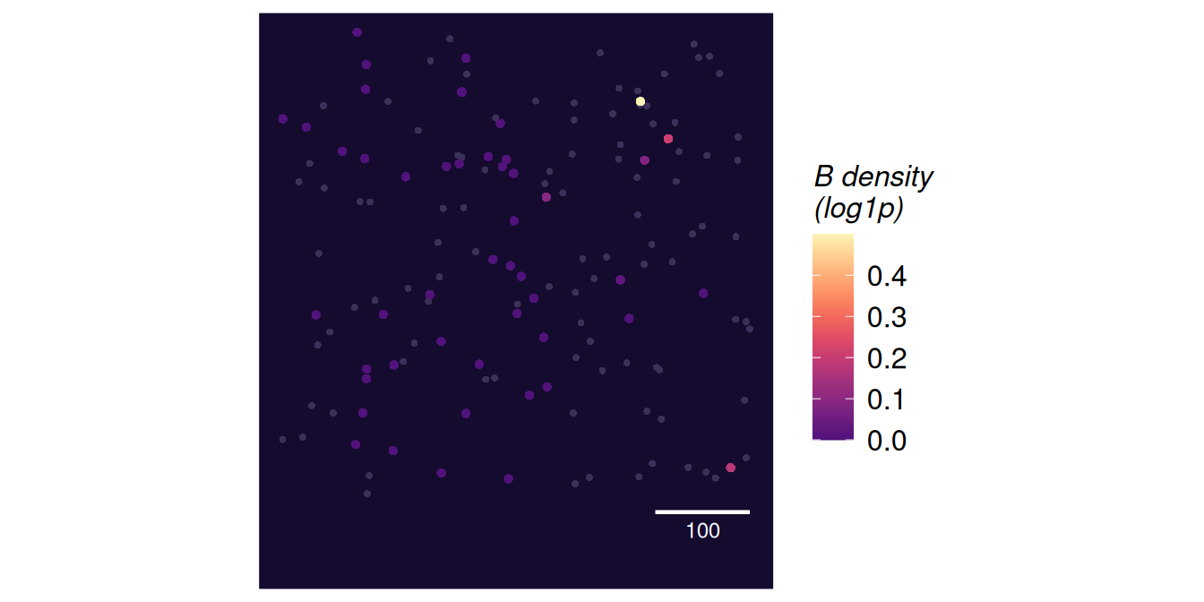
plotNicheMap(spe2, niche = "B", sample = "S1", index = "A", sigma = 30)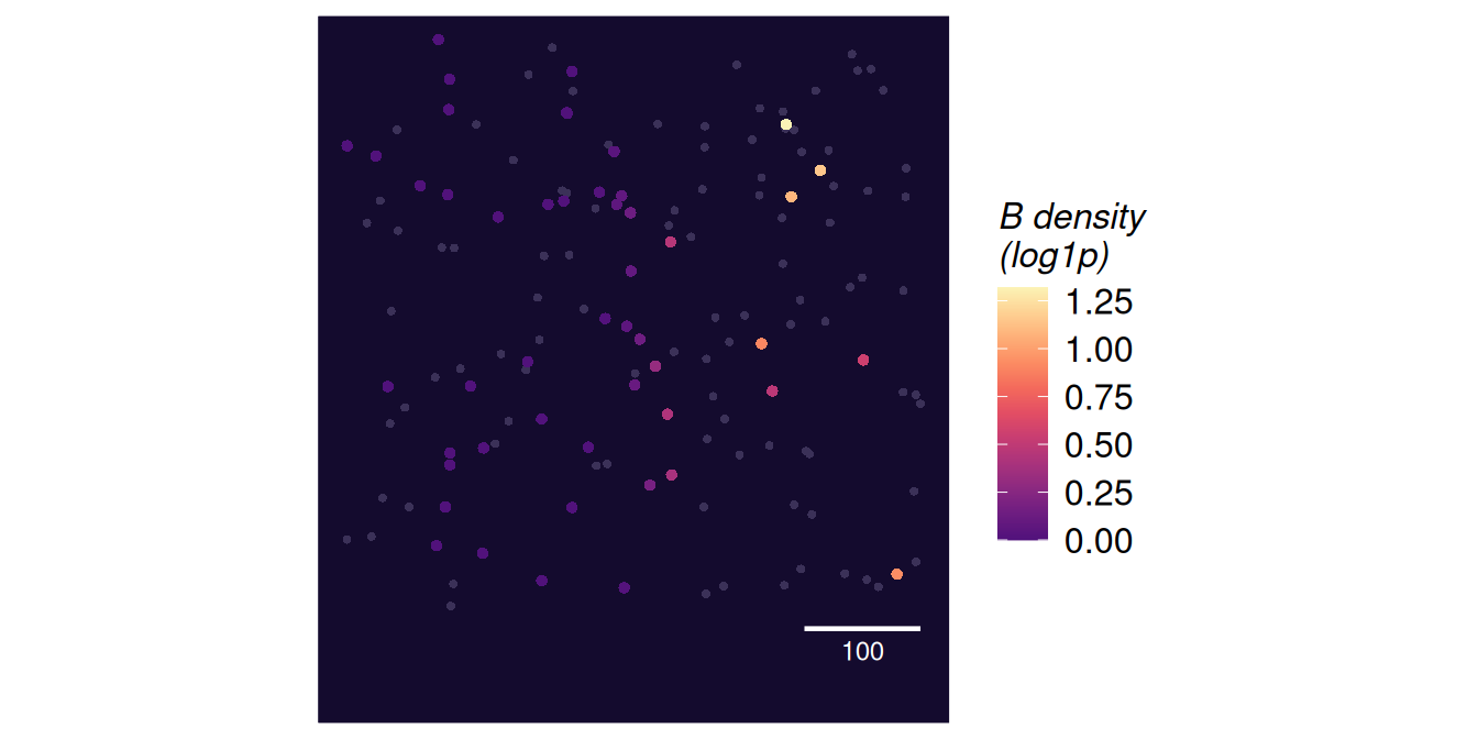
adata10 = sp.build_niches(adata, sigma=10, copy=True)
fig = sp.pl.plot_niche_map(adata10, niche="B", sample="S1", index="A", sigma=10)
plt.show()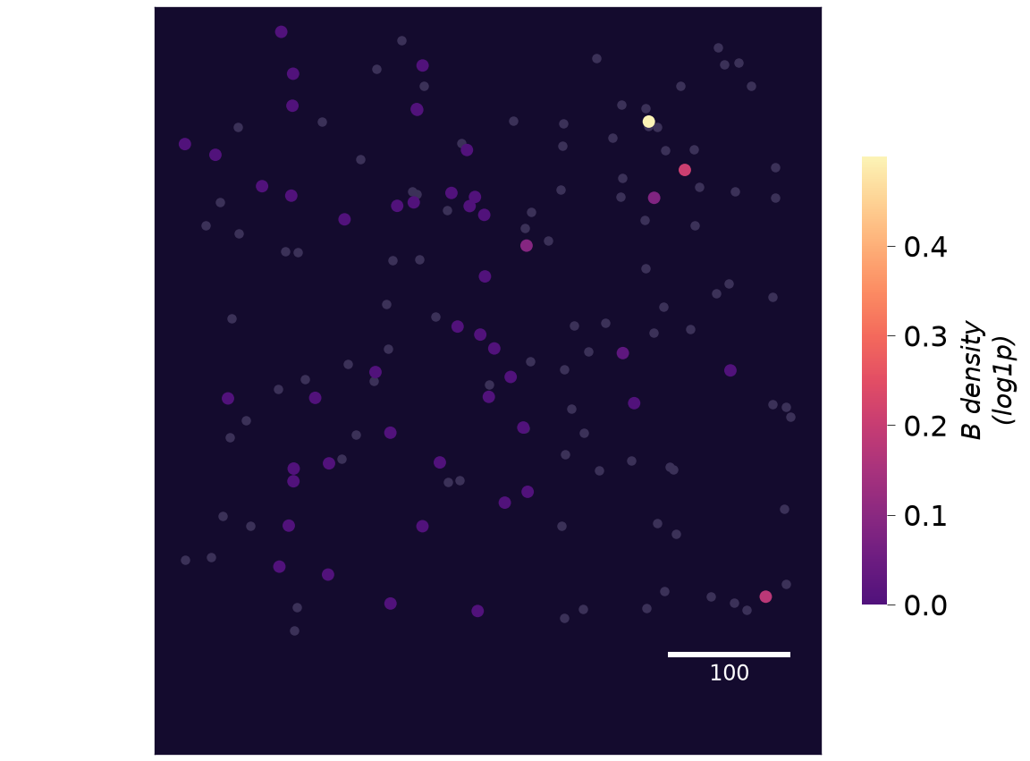
fig = sp.pl.plot_niche_map(adata10, niche="B", sample="S1", index="A", sigma=30)
plt.show()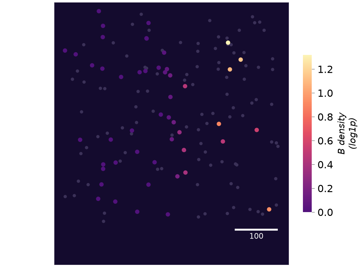
At the smaller bandwidth most cells have no niche cell of type B within reach and the density is zero, so the map is speckled by the position of single cells. At the larger one the density varies smoothly across the section, and we can see where B cells are concentrated. We use 30 for the rest of this page. For real data, choose the bandwidth from what you know about the biology, such as the distance over which cells signal to one another, and from maps like these. mergeNiches() (merge_niches()) can pool several cell types into one niche group (all lymphocytes, say) before fitting. spiDE never tests an index type against its own niche, merged or not.
Fit the model
The fit takes the object with its niches, the bandwidth to use and, if we want to test a condition, the name of the condition column.
fit <- fitSpiDE(spe, condition = "condition", sigma = 30, verbose = FALSE)
fit
#> SpiDEFit (slopes engine), bandwidth 30
#>   16 patients; condition: condition
#>   index A: 20 genes x 2 niches (B, C)
#>   index B: 20 genes x 2 niches (A, C)
#>   index C: 20 genes x 2 niches (A, B)
fit = sp.fit_spide(adata, condition="condition", sigma=30, verbose=False)
fit
#> SpiDEFit (slopes engine), bandwidth 30
#> 16 patients; condition: condition
#> index A: 20 genes x 2 niches (B, C)
#> index B: 20 genes x 2 niches (A, C)
#> index C: 20 genes x 2 niches (A, B)By default every cell type with at least min.cells cells in at least min.patients patients is an index type (min_cells and min_patients in Python), and every other cell type is tested as its niche. The index and niche arguments restrict this; niche types that are not tested stay in the model as adjustments. Genes detected in fewer than min.detect of an index type’s cells are not tested in it. The model adjusts for sequencing depth with the centred log library size of each cell, and further cell-level measurements such as cell area can be added with covariates. Python keeps R’s argument names in snake_case, so min.cells is min_cells.
The engine argument chooses how the error between patients is estimated. The default, "slopes", fits the model once without the condition and then estimates every patient’s own slope for every niche, each with a variance that allows for spatially correlated cells. Because the fit never sees the condition, any patient-level condition can be tested afterwards, and permuting the condition reruns only the test. The alternative, "sandwich", fits the condition-specific model directly, tests its coefficients with a patient-clustered sandwich standard error and needs the condition at fit time. The slopes engine is the more powerful of the two when effects vary between patients, and it is needed for spiGSEA(). The spiDE model explains both engines.
Test the slopes
The test combines the patients’ slopes. It always runs the pooled test, and it runs the condition-specific test when a condition is available, here the one recorded by the fit. A condition can also be given to testSpiDE() (test_spide()) directly.
res <- testSpiDE(fit)
res
#> SpiDEResults (slopes engine)
#>   pooled across patients: 120 tests, 2 at FDR 0.05
#>   condition-specific (Responder - Non-responder; pooled_or_heterogeneity family): 2 tests, 1 at FDR 0.05
res = sp.test_spide(fit)
print(res)
#> SpiDEResults (slopes engine)
#> pooled across patients: 120 tests, 2 at FDR 0.05
#> condition-specific (Responder - Non-responder; pooled_or_heterogeneity family): 2 tests, 1 at FDR 0.05The pooled test
The pooled results are a table with one row per triplet; results(res, test = "pooled") gives it in R and sp.results(res, test="pooled") in Python. estimate is the average within-patient slope on the natural-log scale per unit of the log1p niche density, t and p are the test statistic and its p-value, and q is the q-value after a Benjamini-Hochberg correction over every triplet.
head(results(res, test = "pooled"))sp.results(res, test="pooled").head()
#> gene index niche ... p.heterogeneity q in_family
#> 0 G1 A B ... 0.554557 8.234284e-09 True
#> 1 G9 A B ... 0.254027 1.676479e-03 True
#> 2 G8 B C ... 0.103677 5.685822e-02 True
#> 3 G18 A B ... 0.884934 2.443776e-01 True
#> 4 G2 A B ... 0.259633 4.198921e-01 True
#>
#> [5 rows x 13 columns]The planted triplet, G1 in A against B, comes out as the strongest pooled association, with a t of 6.83 in R. Remember that a pooled call says that, within a patient, index cells with more of the niche type around them express more (or less) of the gene, consistently across patients.
The condition-specific test
The condition-specific table has the same layout. Its estimate is the difference between the conditions in the average slope, the second level minus the first, and res$contrast (res.contrast) says which two levels were compared.
res$contrast
#> [1] "Responder - Non-responder"
cond <- results(res, test = "condition")
cond[cond$in_family, ]print(res.contrast)
#> Responder - Non-responder
cond = sp.results(res, test="condition")
cond[cond["in_family"]]
#> gene index niche ... p.heterogeneity q in_family
#> 1 G1 A B ... 0.554557 0.020112 True
#> 33 G9 A B ... 0.254027 0.272419 True
#>
#> [2 rows x 13 columns]By default the condition-specific test is carried out only among the triplets that pass the pooled test, or whose slopes vary between patients more than their sampling noise allows (p.heterogeneity, corrected at the same fdr). Neither filter looks at the condition, so the correction for multiple testing is spent on triplets that have something for the condition to explain, and the result is valid under any relabelling of the patients. Rows outside this family have q = NA (NaN in Python). Other families are available through the procedure argument: "heterogeneity" and "filtered" use one filter each, and "all" tests every triplet.
In the table, the planted slope is larger in responders than in non-responders by 0.27 log units per unit of log1p density in R (q = 0.02), which is the effect we planted. The whole pipeline can also be run in one call:
res <- spiDE(toySpiDE, condition = "condition", sigma = 30)spide() builds the niche matrix itself and does not keep it on the object (name= is the obsm prefix the niches are read from, or built into):
res2 = sp.spide(sp.datasets.toy_spide(), condition="condition", sigma=30, verbose=False)
print(res2)
#> SpiDEResults (slopes engine)
#>   pooled across patients: 120 tests, 2 at FDR 0.05
#>   condition-specific (Responder - Non-responder; pooled_or_heterogeneity family): 2 tests, 1 at FDR 0.05
Look at the patients behind a result
A call is only as good as the patients behind it. With the slopes engine, every patient has its own slope for every triplet, and these slopes are the evidence that the tests weigh. patientSlopes() (patient_slopes()) returns them as a table, with the slope’s variance and the number of cells that went into it.
ps <- patientSlopes(fit, gene = "G1", index = "A", niche = "B")
head(ps[, c("patient", "condition", "slope", "var_spatial", "ncells")])
ps = sp.patient_slopes(fit, gene="G1", index="A", niche="B")
ps[["patient", "condition", "slope", "var_spatial", "ncells"]].head()
#> patient condition slope var_spatial ncells
#> 0 S1 Responder 0.465072 0.008294 49
#> 1 S10 Non-responder 0.176669 0.059603 61
#> 2 S11 Responder 0.400428 0.010850 60
#> 3 S12 Non-responder 0.204428 0.084545 41
#> 4 S13 Responder 0.401380 0.021371 54plotPatientSlopes() (pl.plot_patient_slopes()) draws them. Each point is a patient’s slope with its interval, sized by the weight the patient carries in the tests. The weighted average of each condition is marked, and the pooled estimate is shown as a band.
plotPatientSlopes(res, gene = c("G1", "G2"), index = "A", niche = "B")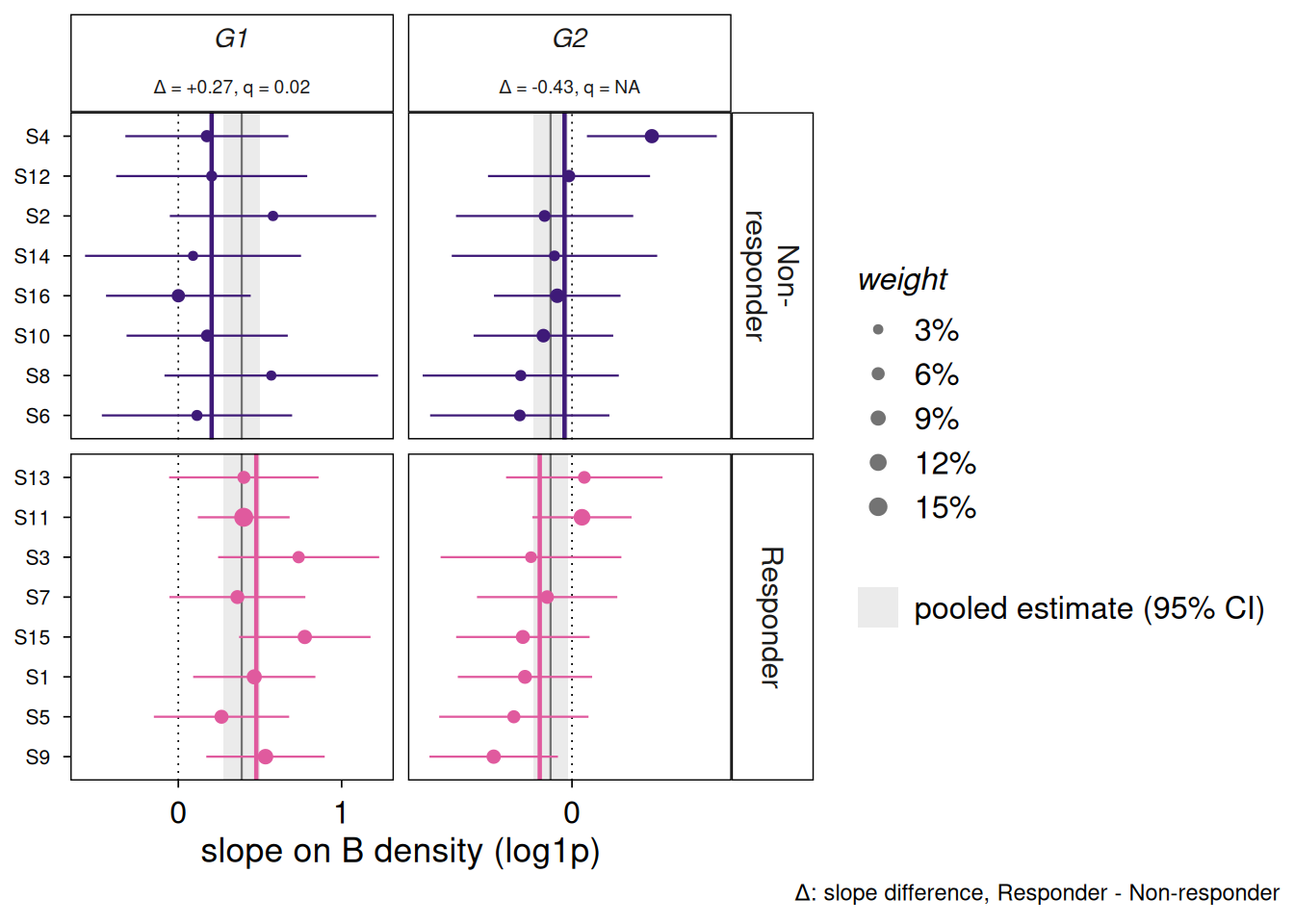
fig = sp.pl.plot_patient_slopes(res, gene=["G1", "G2"], index="A", niche="B")
plt.show()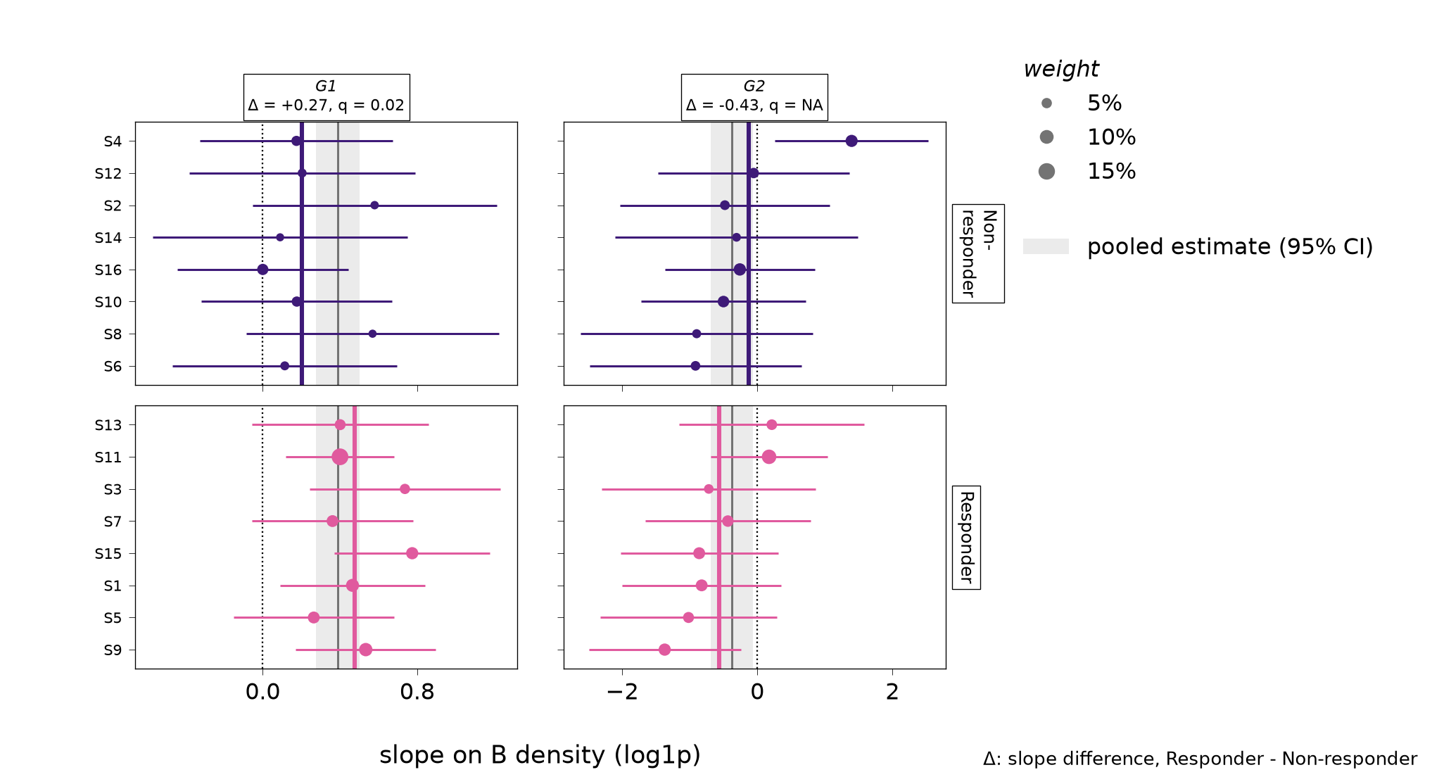
For G1, the slopes of the patients lie mostly above zero in both conditions, which gives the pooled call, and the slopes of the responders sit further to the right than those of the non-responders, which is what the condition-specific test picks up. The panel title reports its difference and q-value. For G2, which has no planted effect, the slopes are spread widely on both sides of zero, their intervals are wide, and the two conditions overlap.
The model also gives each patient a baseline level of every gene, its intercept. These baselines absorb everything that differs between patients as a whole, so they are not tested, but they are worth a look. patientIntercepts() (patient_intercepts()) returns them with the patient-level covariates, and plotPatientEffects() (pl.plot_patient_effects()) summarises them by principal components of the intercepts, showing how much of each component each covariate explains.
intercepts <- patientIntercepts(fit, gene = "G1", index = "A")
head(intercepts)plotPatientEffects(res, index = "A")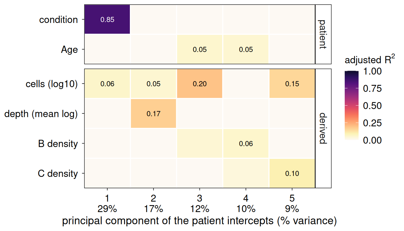
intercepts = sp.patient_intercepts(fit, gene="G1", index="A")
intercepts.head()
#>   gene index patient  intercept  ncells sample_id      condition       Age
#> 0   G1     A      S1   2.185319      49        S1      Responder  0.525262
#> 1   G1     A     S10   1.782854      61       S10  Non-responder -2.566746
#> 2   G1     A     S11   2.157735      60       S11      Responder  1.213412
#> 3   G1     A     S12   1.627117      41       S12  Non-responder  0.362418
#> 4   G1     A     S13   2.223423      54       S13      Responder -1.853804
fig = sp.pl.plot_patient_effects(res, index="A")
plt.show()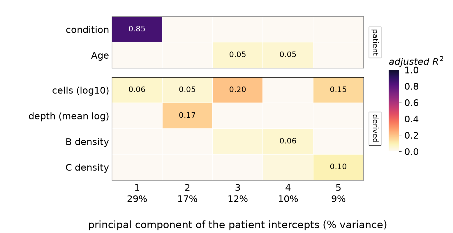
In this example the first component of the intercepts lines up almost entirely with the condition, which is what we expect: the baselines absorb the difference in level between responders and non-responders, so that this difference cannot be mistaken for a difference in slope. Other covariates, such as the number of cells and the depth of a patient, explain smaller parts of the other components. If a slide or batch column lined up with a component of the slopes instead, the condition would be partly confounded with it, and that column should go into strata. Setting niche in the plot function draws the same plot for the slopes, which is the check to make before trusting a condition-specific call.
Test gene sets
Genes do not act alone, and a set of genes with a shared function often shows an effect that no single gene shows clearly. spiGSEA() (spi_gsea()) tests gene sets in the way the gene test tests genes. It takes the results and any named list (a dict in Python) of gene symbols, such as the collections of the msigdb package. Each patient gets a slope for the set, which averages its genes’ slopes after putting them on a common scale, and these set slopes go through the same pooled and condition-specific tests. By default (type = "competitive") the average over the other tested genes is subtracted, so a set is called when it moves more than the typical gene. It needs the slopes engine.
sets <- list(planted = c("G1", "G2", "G3"), other = paste0("G", 4:8),
             rest = paste0("G", 9:20))
gs <- spiGSEA(res, sets, min.size = 3)
head(gs[, c("set", "index", "niche", "test", "size", "estimate", "p", "q", "q.global")])
sets = {
"planted": ["G1", "G2", "G3"],
"other": [f"G{i}" for i in range(4, 9)],
"rest": [f"G{i}" for i in range(9, 21)],
}
gs = sp.spi_gsea(res, sets, min_size=3)
gs[["set", "index", "niche", "test", "size", "estimate", "p", "q", "q.global"]].head()
#> set index niche test size estimate p q q.global
#> 0 planted A B pooled 3 0.578673 0.000011 0.000032 0.000191
#> 1 planted C A pooled 3 0.237550 0.045308 0.135925 0.233513
#> 2 other B C pooled 5 -0.215171 0.048372 0.145115 0.233513
#> 3 planted B A pooled 3 0.270073 0.051892 0.155676 0.233513
#> 4 rest A B pooled 12 -0.195542 0.094970 0.142454 0.341890There are two q-values. q adjusts within each (index, niche, test) column, and q.global over every set, index and niche of a test. When there are many sets and many columns, q.global is the one to read. The heatmap shows the t statistic of every set in every (index, niche) column, with a dot where q.global passes.
plotTripletHeatmap(gs, test = "pooled")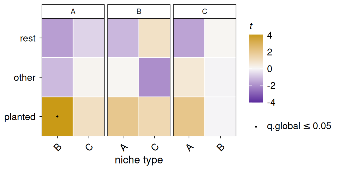
fig = sp.pl.plot_triplet_heatmap(gs, test="pooled")
plt.show()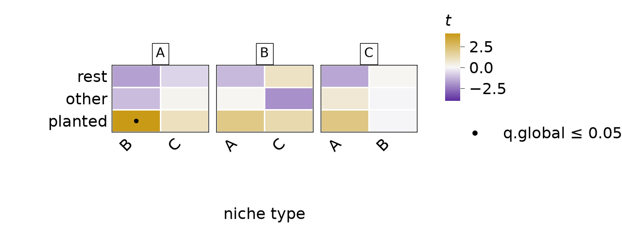
The set holding the planted gene stands out in the column of A against B, where it is called, and no other set is called.
A different question: niche abundance
The tests above use only the slopes within patients. A patient whose index cells sit among many niche cells may also express a gene differently as a whole from a patient whose index cells do not. This is a real association, but it is a different claim. It says that patients with more of a niche type differ, not that a cell responds to its neighbours, and the patient intercepts absorb it so that the slope test never sees it. testNicheAbundance() (test_niche_abundance()) asks it directly. For each patient and index type it forms a pseudobulk profile and compares it with the patient’s average niche density, across patients.
ab <- testNicheAbundance(spe, condition = "condition", sigma = 30, verbose = FALSE)
head(ab)
ab = sp.test_niche_abundance(adata, condition="condition", sigma=30, verbose=False)
ab.head()
#> gene index niche term ... leverage downweighted q q.global
#> 0 G1 A B niche ... 3.140745 1 0.770461 0.945496
#> 1 G2 A B niche ... 3.140745 1 0.770461 0.907598
#> 2 G3 A B niche ... 3.140745 1 0.770461 0.662375
#> 3 G4 A B niche ... 3.140745 1 0.770461 0.907598
#> 4 G5 A B niche ... 3.140745 1 0.770461 0.737781
#>
#> [5 rows x 12 columns]With a condition, the rows with term "niche" give the association averaged over the two conditions, and the rows with "condition:niche" test whether it differs between them, again the second level minus the first. Each term is its own family for multiple testing, with its own q.global. A patient who alone carries most of a niche type’s spread is down-weighted (max.leverage, max_leverage in Python), so that one patient cannot make a call on its own. Gene sets go through the same test with the genesets argument.
The two kinds of result must not be mixed up, and never report a result of one test as a result of the other. A slope result says that, within a patient, cells with more of this niche differ, and an abundance result says that patients with more of this niche differ. plotNicheResponse() (pl.plot_niche_response()) shows both on one gene. With adjust = FALSE (adjust=False) it draws the raw data: each segment is one patient’s slope, the quantity spiDE tests, and the dashed line through the patients’ means is the between-patient association that the abundance test tests.
plotNicheResponse(spe, res, gene = "G1", index = "A", niche = "B", adjust = FALSE)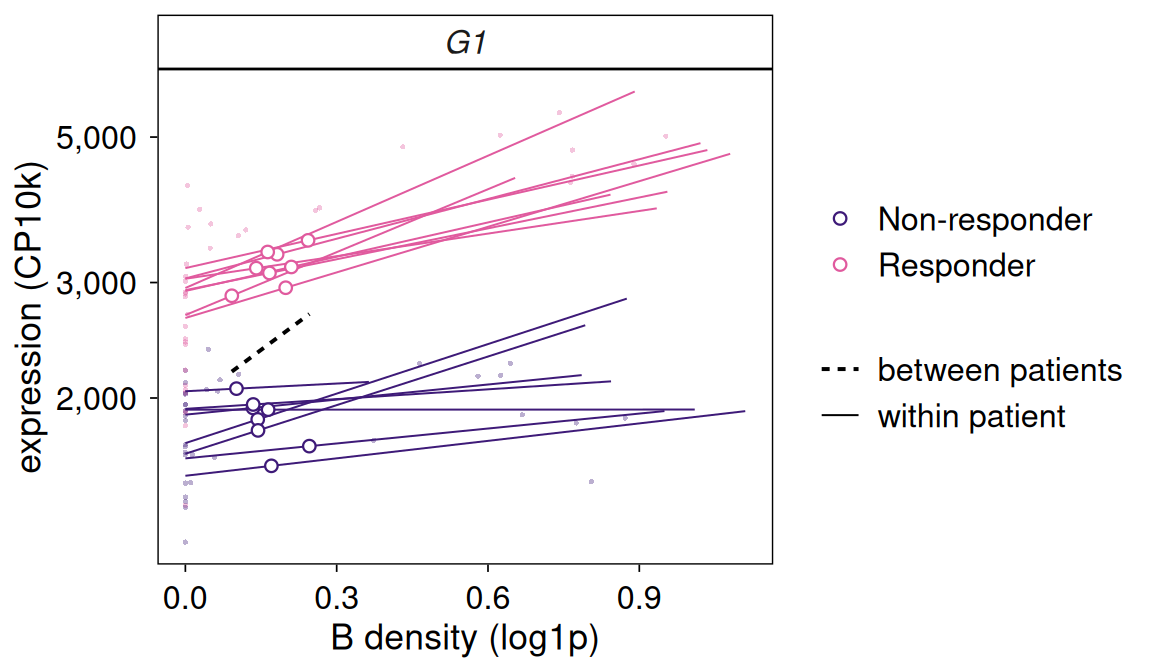
fig = sp.pl.plot_niche_response(adata, res, gene="G1", index="A", niche="B", adjust=False)
plt.show()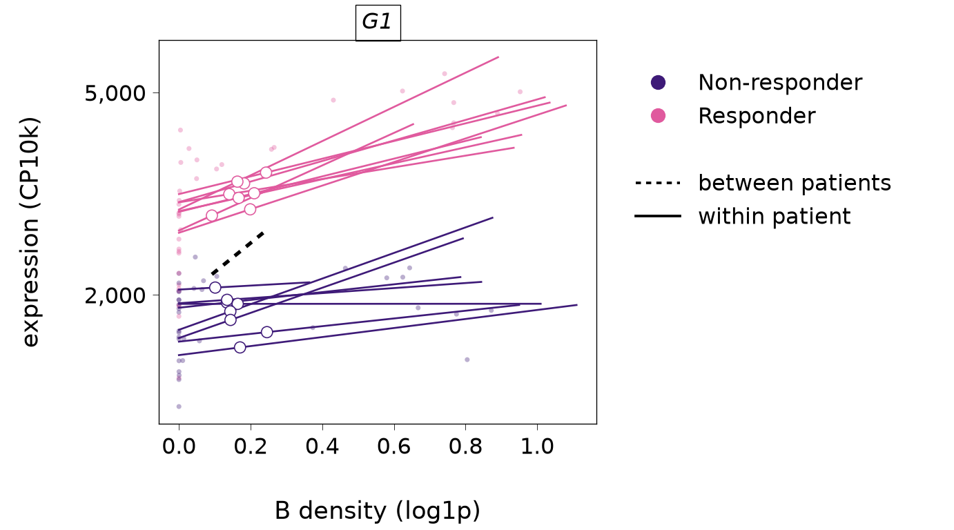
Within a patient the segments rise with the density of B, more steeply for some patients than for others, while the dashed line across the patients’ means is the different, between-patient question.
Plots
All the plots are in one house style with one colour-blind-safe palette (theme_spiDE() and spiDEColours() in R, pl.style() and pl.spide_colours() in Python) that uses one pair of colours for slopes that rise or fall with the niche and another pair for the two levels of the condition. In R every plot is a ggplot2 object that returns its data in p$data, so a plot is changed by adding layers or a theme, and any two plots can be combined with patchwork. In Python every plot is a matplotlib Figure.
Where the calls are
plotCallMap() (pl.plot_call_map()) counts, for each (index, niche) column, how many triplets pass, separately for slopes that rise and slopes that fall with the niche’s density, and plotTopTriplets() (pl.plot_top_triplets()) shows the strongest ones. When we give it the data object, a triangle marks a gene that is several-fold higher in the niche type than in the index type, which we come back to below.
plotCallMap(res, test = "pooled")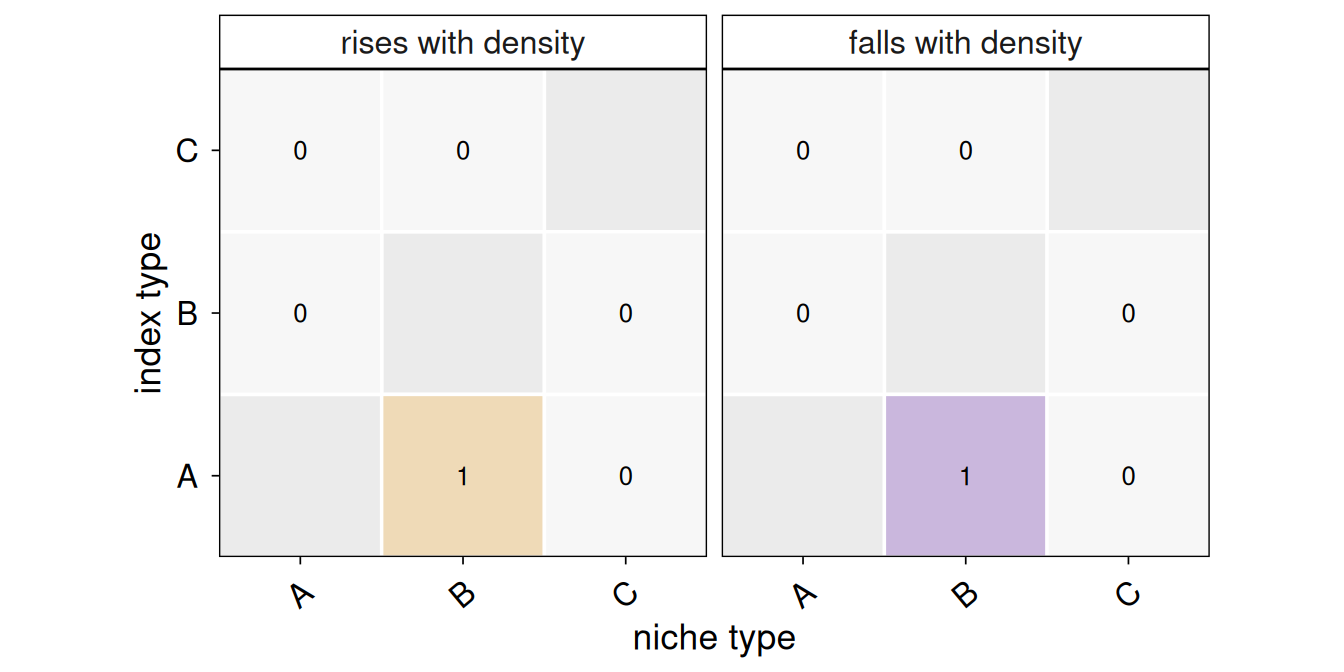
plotTopTriplets(res, test = "pooled", n = 12, spe = spe)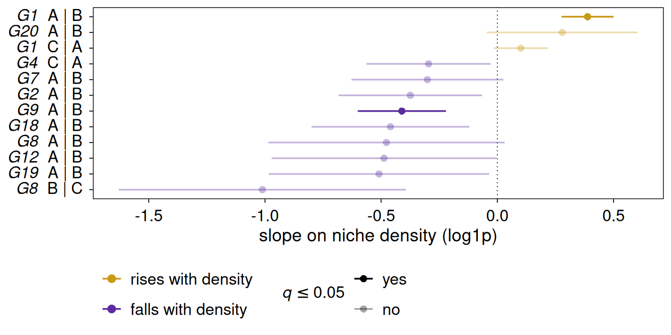
fig = sp.pl.plot_call_map(res, test="pooled")
plt.show()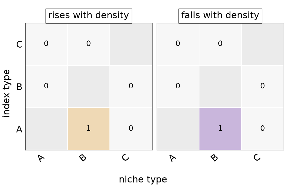
fig = sp.pl.plot_top_triplets(res, test="pooled", n=12, adata=adata)
plt.show()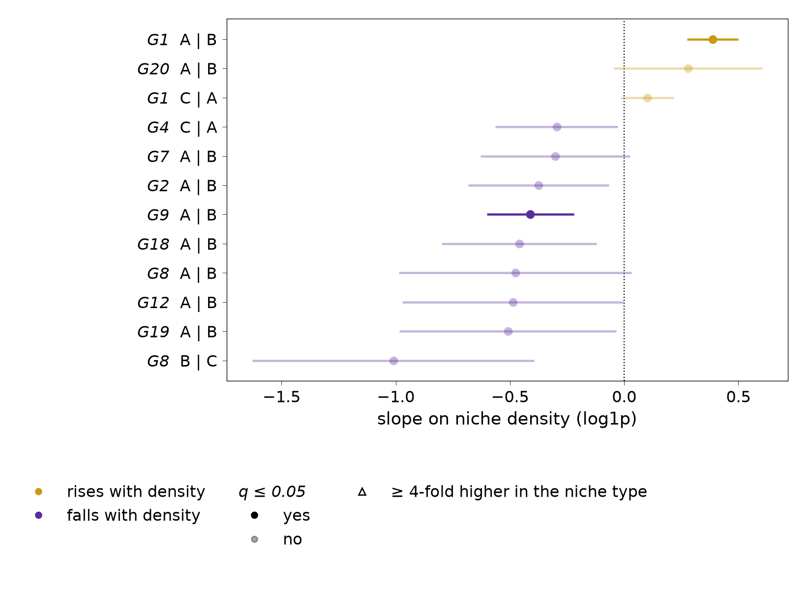
Two triplets pass, both in the column of index type A against niche type B, where the effect was planted: the planted gene G1, whose slope rises, and G9, whose slope falls. G9 has no planted effect, so it is an unplanted call at the default threshold, which is what we should expect to see now and then among 120 triplets.
The cells behind a slope
plotNicheResponse() shows the cells themselves. By default, each patient’s fitted intercept is divided out, so the patients share one level and the slopes that the tests compare are easy to see.
plotNicheResponse(spe, res, gene = c("G1", "G2"), index = "A", niche = "B")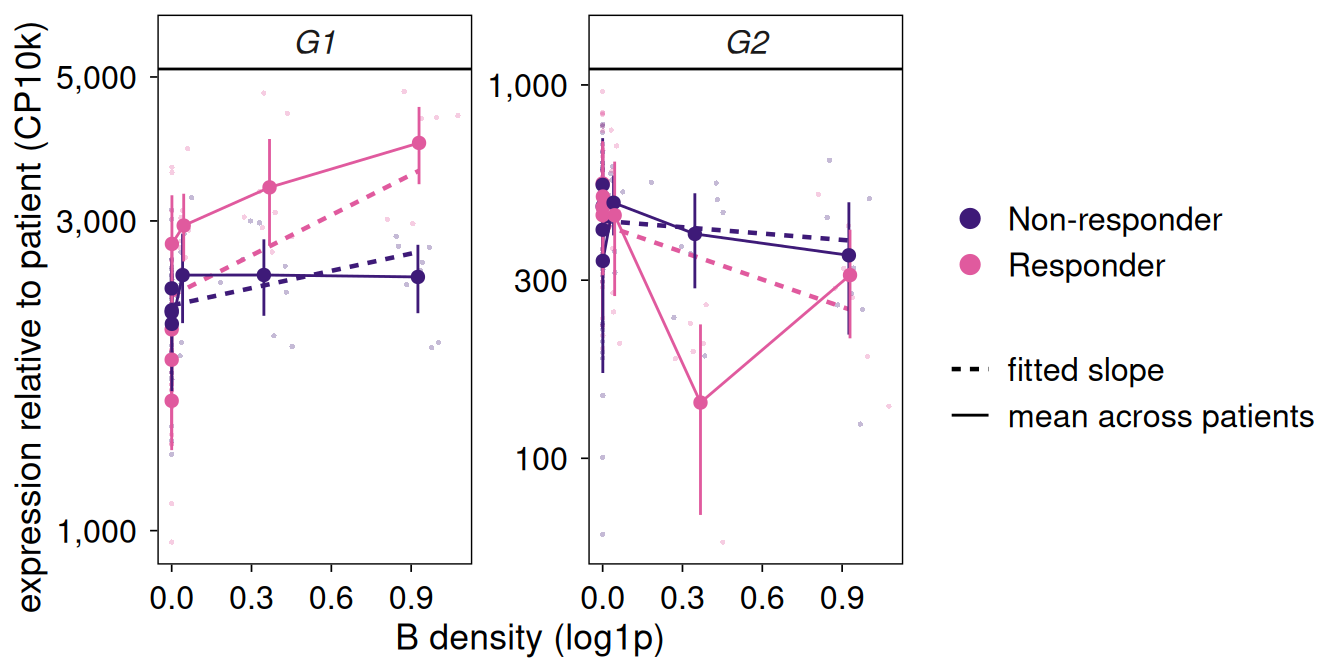
fig = sp.pl.plot_niche_response(adata, res, gene=["G1", "G2"], index="A", niche="B")
plt.show()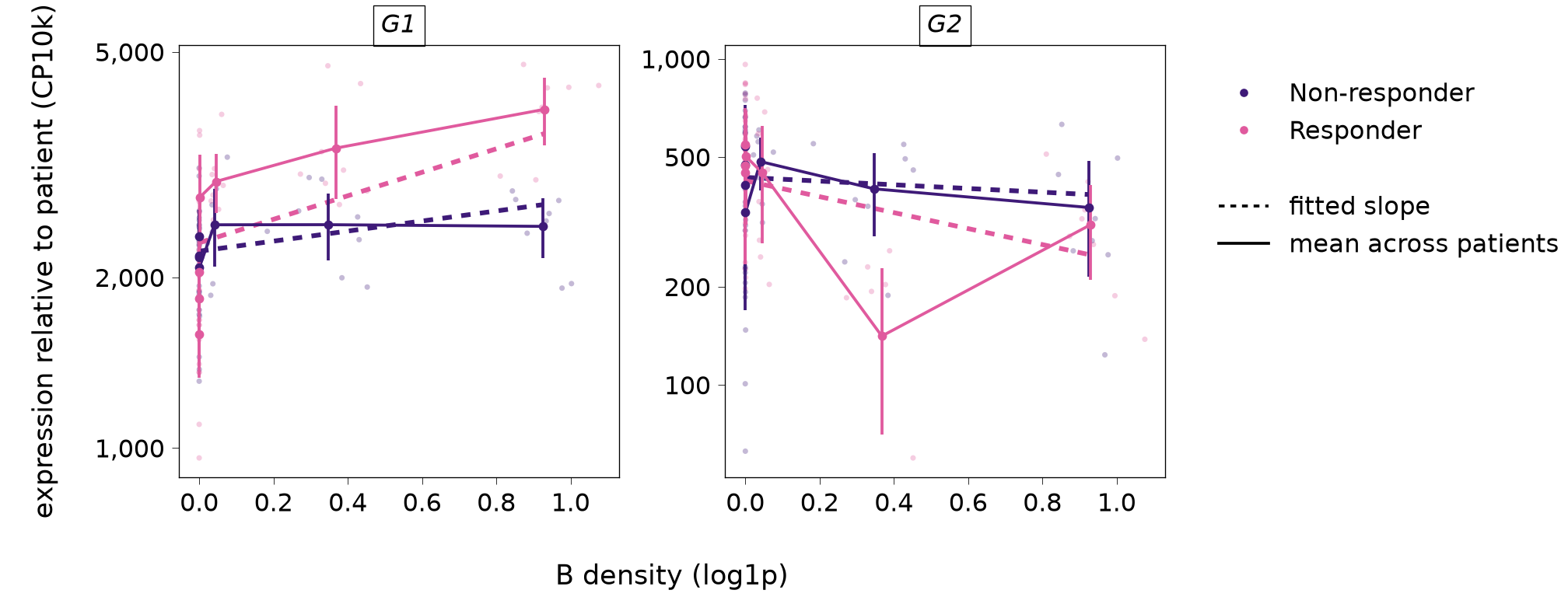
For G1, the expression of the responders’ cells rises with the density of B while that of the non-responders is nearly flat. For G2, there is no clear trend in either group.
Check for spillover
Cell segmentation is never perfect, and transcripts of a neighbouring niche cell can be assigned to an index cell. These transcripts rise with the niche’s density and look like a response of the index cell. plotSpillover() (pl.plot_spillover()) plots every triplet by its signed z statistic against how much higher the gene is in the niche type than in the index type, and marks the region of genes that are several-fold higher in the niche type. If the calls fell mostly in that region, they would be the niche type’s own markers and spillover the likely explanation.
plotSpillover(res, spe)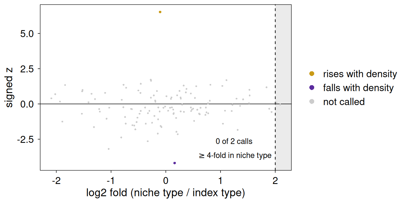
fig = sp.pl.plot_spillover(res, adata)
plt.show()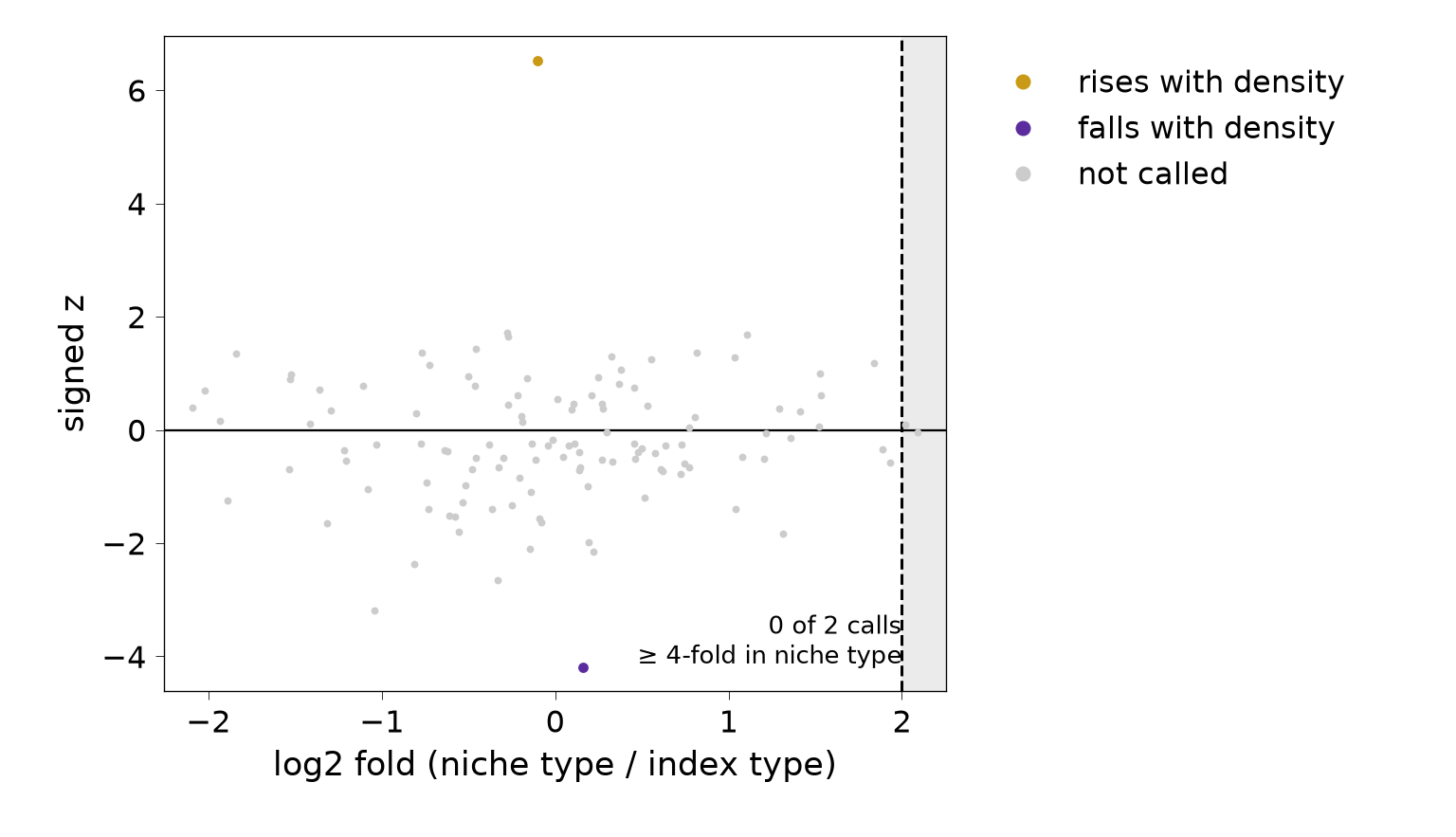
In this example none of the calls lies in that region, so spillover does not explain them. In real data, report the niche type’s fold change together with every call.
Diagnostics
plotPValues() (pl.plot_p_values()) shows the distribution of the p-values by expression band. It is a sanity check on the data at hand and is not a replacement for the calibration checks of Validation.
plotPValues(res)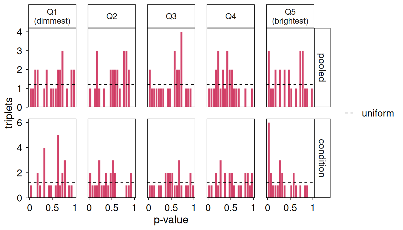
fig = sp.pl.plot_p_values(res)
plt.show()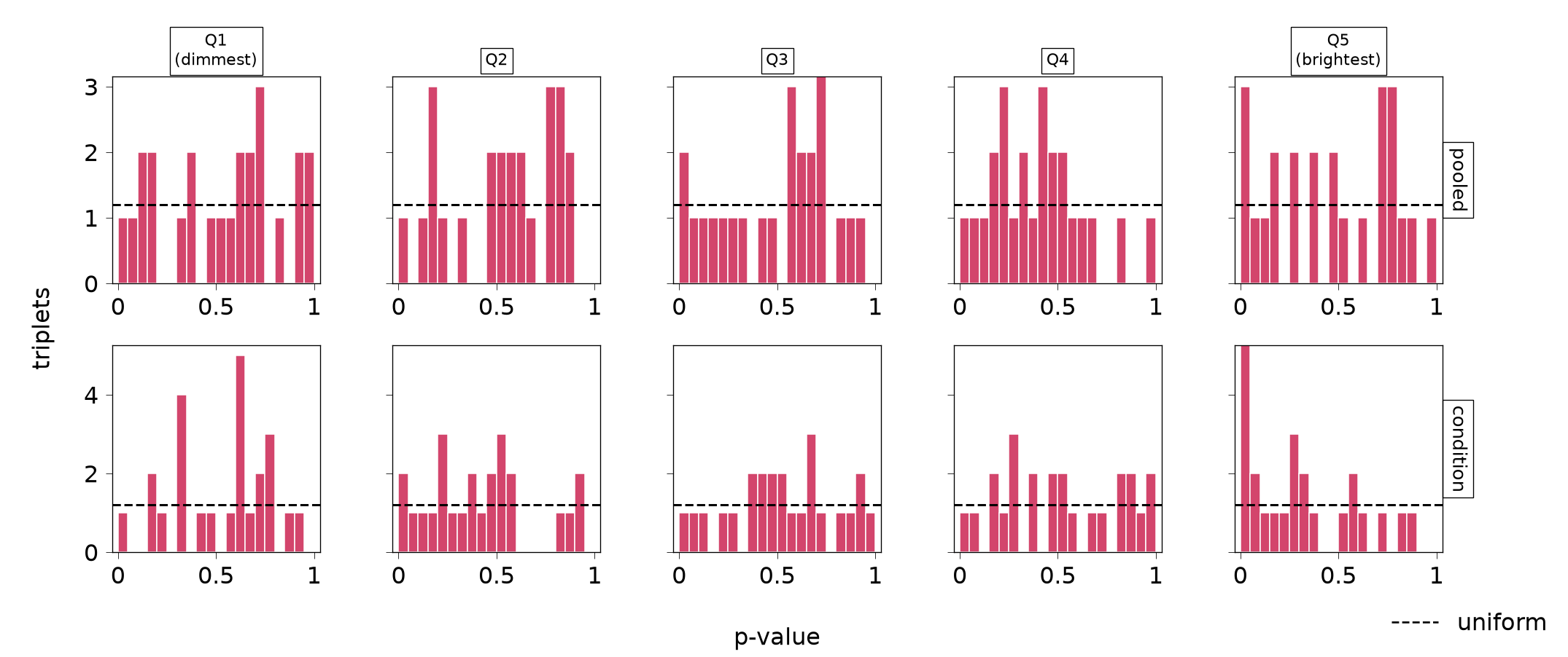
With only 20 genes per band the histograms are coarse, and the p-values are spread across the range with no strong pile-up near zero in any band, which is what a data set with one planted effect should look like.
In R, figures combine with patchwork, for example to put a patient-level and a cell-level view of the same triplet side by side. Python figures are independent matplotlib objects with no counterpart of this operator, so we show the two in turn.
library(patchwork)
plotPatientSlopes(res, gene = "G1", index = "A", niche = "B") +
  plotNicheResponse(spe, res, gene = "G1", index = "A", niche = "B") +
  plot_annotation(tag_levels = "A")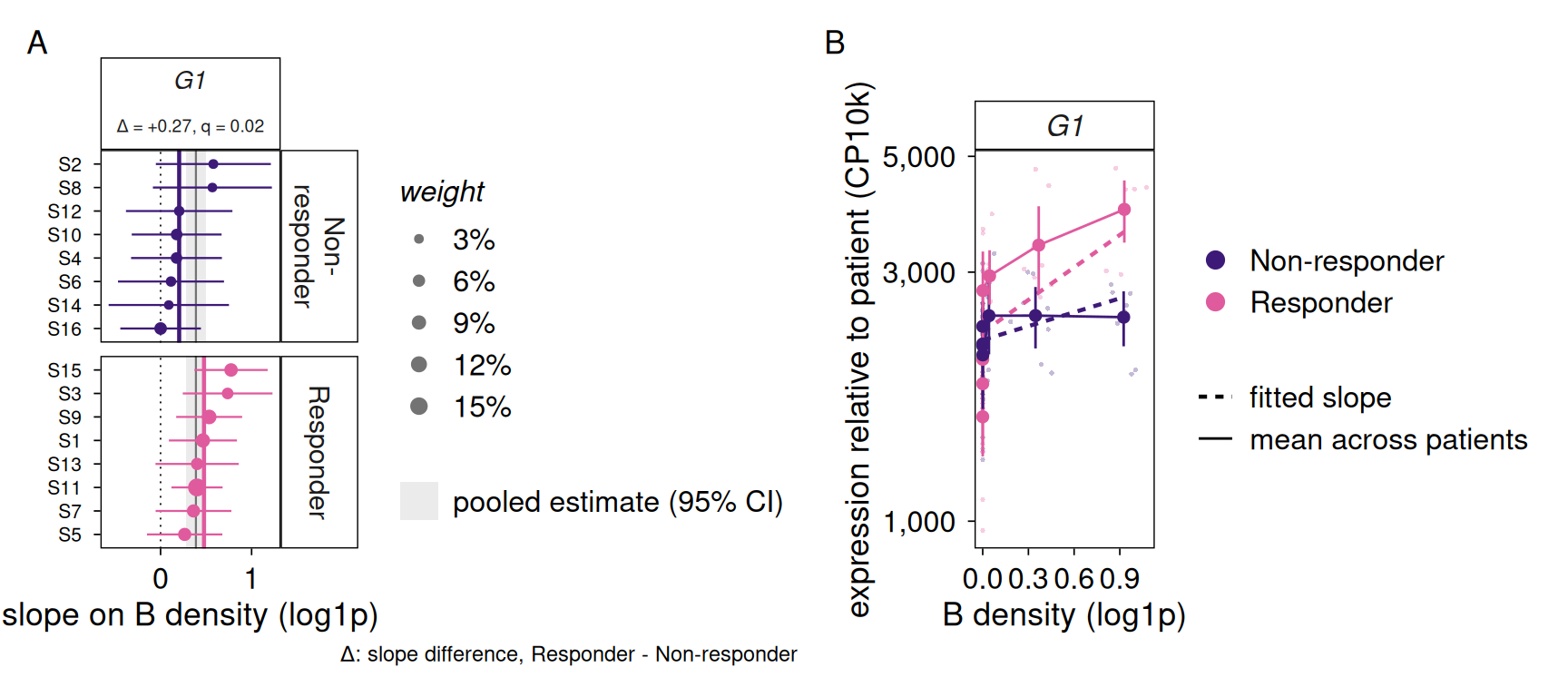
fig = sp.pl.plot_patient_slopes(res, gene="G1", index="A", niche="B")
plt.show()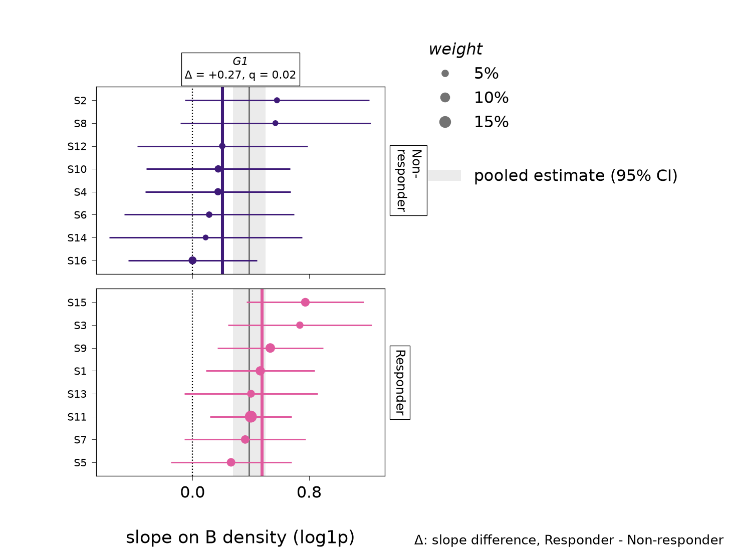
fig = sp.pl.plot_niche_response(adata, res, gene="G1", index="A", niche="B")
plt.show()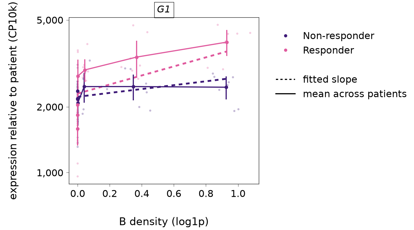
Practicalities
Runtime. The fit is the expensive step. Every gene is fitted separately in every index type, so the time grows with the number of index types, the number of genes and the number of cells, but it hardly depends on the number of patients, because the patient baselines are handled algebraically. The example above takes a few seconds. Testing is fast, and a permutation of the condition under the slopes engine reruns only the test.
Parallelism. Genes are fitted independently within an index type, so they can be spread over workers: with the BPPARAM argument in R and n_jobs in Python. Results are identical for any n_jobs.
library(BiocParallel)
fit <- fitSpiDE(spe, condition = "condition", sigma = 30,
                BPPARAM = MulticoreParam(4))
fit = sp.fit_spide(adata, condition="condition", sigma=30, n_jobs=4)Forked workers in R run one BLAS thread each when the RhpcBLASctl package is installed. Otherwise, set OMP_NUM_THREADS=1 in the job, because workers that each use many threads compete with one another and run much slower.
Counts and sparsity. Counts must be integers, and a back-transformed normalised layer is refused. In Python layers["counts"] can be a CSR or CSC sparse matrix and gives the same results as dense.
Several bandwidths. One fit uses one bandwidth. We can build the niches at several bandwidths and fit each one, but the results are a sensitivity analysis and not a search: each bandwidth is its own set of tests, and picking the best of them after looking would not be valid. Calls that hold at both bandwidths are the more convincing. Below we refit index type A at the smaller bandwidth and count the pooled calls at each bandwidth.
fit10 <- fitSpiDE(spe2, condition = "condition", sigma = 10, index = "A",
                  verbose = FALSE)
res10 <- testSpiDE(fit10)
r10 <- results(res10, test = "pooled")
r30 <- results(res, test = "pooled")
r30 <- r30[r30$index == "A", ]
c(sigma10 = sum(r10$q < 0.05, na.rm = TRUE), sigma30 = sum(r30$q < 0.05, na.rm = TRUE))
#> sigma10 sigma30
#>       3       2
fit10 = sp.fit_spide(adata10, condition="condition", sigma=10, index="A", verbose=False)
r10 = sp.results(sp.test_spide(fit10), test="pooled")
r30 = sp.results(res, test="pooled")
r30 = r30[r30["index"] == "A"]
print({"sigma10": int((r10["q"] < 0.05).sum()), "sigma30": int((r30["q"] < 0.05).sum())})
#> {'sigma10': 3, 'sigma30': 2}Both bandwidths call a handful of triplets in A, including the planted one, so the conclusion does not hinge on the choice here.
Objects from older versions. Objects saved by spiDE 0.99.22 and earlier came from a different model and are refused by this version, with a message that names the archive that reads them.
Do R and Python agree?
spidepy is a port of the R package, and a test suite compares it with reference values computed by R, but the two are separate implementations, so we do not take agreement for granted. Here we compare the tables that the two have just produced on the same data: the pooled and condition-specific slope tests, the gene-set test and the niche-abundance test.
as_r_table <- function(code) {
  d <- reticulate::py_to_r(reticulate::py_eval(code, convert = FALSE))
  as.data.frame(lapply(d, unlist), stringsAsFactors = FALSE)
}
key <- function(d) paste(d$gene, d$index, d$niche, d$term, d$set, d$test)
cmp <- function(r, p, col) {
  p <- p[match(key(r), key(p)), ]
  c(max_abs_diff = max(abs(r[[col]] - p[[col]]), na.rm = TRUE),
    max_rel_diff = max(abs(r[[col]] - p[[col]]) / pmax(abs(r[[col]]), 1e-8), na.rm = TRUE))
}
r_pooled <- results(res, test = "pooled")
r_cond <- results(res, test = "condition")
py_pooled <- as_r_table("sp.results(res, test='pooled').to_dict('list')")
py_cond <- as_r_table("sp.results(res, test='condition').to_dict('list')")
py_gs <- as_r_table("gs.to_dict('list')")
py_ab <- as_r_table("ab.to_dict('list')")
out <- rbind(pooled_estimate = cmp(r_pooled, py_pooled, "estimate"),
             pooled_t = cmp(r_pooled, py_pooled, "t"),
             condition_estimate = cmp(r_cond, py_cond, "estimate"),
             gene_set_estimate = cmp(as.data.frame(gs), py_gs, "estimate"),
             abundance_estimate = cmp(as.data.frame(ab), py_ab, "estimate"))
signif(out, 2)
#>                    max_abs_diff max_rel_diff
#> pooled_estimate         1.5e-15      2.4e-14
#> pooled_t                1.4e-14      2.4e-14
#> condition_estimate      2.9e-15      2.3e-14
#> gene_set_estimate       2.2e-15      3.3e-14
#> abundance_estimate      8.1e-14      1.2e-11
calls <- function(d) sort(key(d)[which(d$q < 0.05)])
c(pooled_calls_R = length(calls(r_pooled)), pooled_calls_Python = length(calls(py_pooled)),
  same_pooled_calls = identical(calls(r_pooled), calls(py_pooled)),
  same_condition_family = identical(r_cond$in_family, py_cond$in_family[match(key(r_cond), key(py_cond))]))
#>        pooled_calls_R   pooled_calls_Python     same_pooled_calls
#>                     2                     2                     1
#> same_condition_family
#>                     1
Each row of the table gives the largest absolute and relative difference over all rows between the R and the Python value. On this data they are at the level of floating-point rounding, and the two languages call the same triplets. This is a statement about this example. Real data are larger, the optimisers see more difficult genes, and small differences in the dispersion estimates can reach the last reported digits, so when you compare the two on your own data, compare calls and effect sizes, not digits.
Session information
sessionInfo()
#> R version 4.6.1 (2026-06-24)
#> Platform: x86_64-pc-linux-gnu
#> Running under: Ubuntu 24.04.5 LTS
#>
#> Matrix products: default
#> BLAS:   /usr/lib/x86_64-linux-gnu/openblas-pthread/libblas.so.3
#> LAPACK: /usr/lib/x86_64-linux-gnu/openblas-pthread/libopenblasp-r0.3.26.so;  LAPACK version 3.12.0
#>
#> locale:
#>  [1] LC_CTYPE=C.UTF-8       LC_NUMERIC=C           LC_TIME=C.UTF-8
#>  [4] LC_COLLATE=C.UTF-8     LC_MONETARY=C.UTF-8    LC_MESSAGES=C.UTF-8
#>  [7] LC_PAPER=C.UTF-8       LC_NAME=C              LC_ADDRESS=C
#> [10] LC_TELEPHONE=C         LC_MEASUREMENT=C.UTF-8 LC_IDENTIFICATION=C
#>
#> time zone: UTC
#> tzcode source: system (glibc)
#>
#> attached base packages:
#> [1] stats4    stats     graphics  grDevices utils     datasets  methods
#> [8] base
#>
#> other attached packages:
#>  [1] patchwork_1.3.2             SpatialExperiment_1.23.0
#>  [3] SingleCellExperiment_1.35.2 SummarizedExperiment_1.43.0
#>  [5] Biobase_2.73.2              GenomicRanges_1.65.4
#>  [7] Seqinfo_1.3.2               IRanges_2.47.5
#>  [9] S4Vectors_0.51.10           BiocGenerics_0.59.12
#> [11] generics_0.1.4              MatrixGenerics_1.25.0
#> [13] matrixStats_1.5.0           spiDE_0.99.37
#>
#> loaded via a namespace (and not attached):
#>  [1] gtable_0.3.6           rjson_0.2.23           xfun_0.62
#>  [4] ggplot2_4.0.3          ggrepel_0.9.8          spatstat.sparse_3.2-0
#>  [7] lattice_0.22-9         vctrs_0.7.3            tools_4.6.1
#> [10] spatstat.utils_3.2-5   goftest_1.2-3          parallel_4.6.1
#> [13] tibble_3.3.1           pkgconfig_2.0.3        Matrix_1.7-5
#> [16] RColorBrewer_1.1-3     S7_0.2.2               lifecycle_1.0.5
#> [19] SpaNorm_1.7.16         deldir_2.0-4           compiler_4.6.1
#> [22] farver_2.1.2           RhpcBLASctl_0.23-42    statmod_1.5.2
#> [25] codetools_0.2-20       spatstat.explore_3.8-3 htmltools_0.5.9
#> [28] yaml_2.3.12            pillar_1.11.1          BiocParallel_1.47.0
#> [31] DelayedArray_0.39.8    limma_3.99.2           spatstat.univar_3.2-0
#> [34] magick_2.9.1           abind_1.4-8            nlme_3.1-169
#> [37] spatstat.geom_3.8-3    tidyselect_1.2.1       rsvd_1.0.6
#> [40] digest_0.6.39          BiocSingular_1.29.2    dplyr_1.2.1
#> [43] splines_4.6.1          labeling_0.4.3         polyclip_1.10-7
#> [46] fastmap_1.2.0          grid_4.6.1             cli_3.6.6
#> [49] SparseArray_1.13.4     magrittr_2.0.5         S4Arrays_1.13.2
#> [52] spatstat.data_3.1-9    withr_3.0.3            tensor_1.5.1
#> [55] scales_1.4.0           rmarkdown_2.32         XVector_0.53.0
#> [58] otel_0.2.0             reticulate_1.47.0      png_0.1-9
#> [61] ScaledMatrix_1.21.0    beachmat_2.29.3        evaluate_1.0.5
#> [64] knitr_1.52             irlba_2.4.1            mgcv_1.9-4
#> [67] rlang_1.3.0            Rcpp_1.1.2             spatstat.random_3.5-2
#> [70] glue_1.8.1             jsonlite_2.0.0         R6_2.6.1
import platform
from importlib.metadata import version
pkgs = ["spidepy", "spanormpy", "anndata", "numpy", "pandas", "scipy", "matplotlib"]
print("python", platform.python_version())
#> python 3.12.15
for p in pkgs:
print(p, version(p))
#> spidepy 0.1.0.dev0
#> spanormpy 0.1.0
#> anndata 0.13.4
#> numpy 2.5.4
#> pandas 3.0.6
#> scipy 1.18.1
#> matplotlib 3.11.2