library("spiDE")
data(toySpiDE)
spe <- buildNiches(toySpiDE, sigma = 30)
plotNicheMap(spe, niche = "B", sample = "S1", index = "A")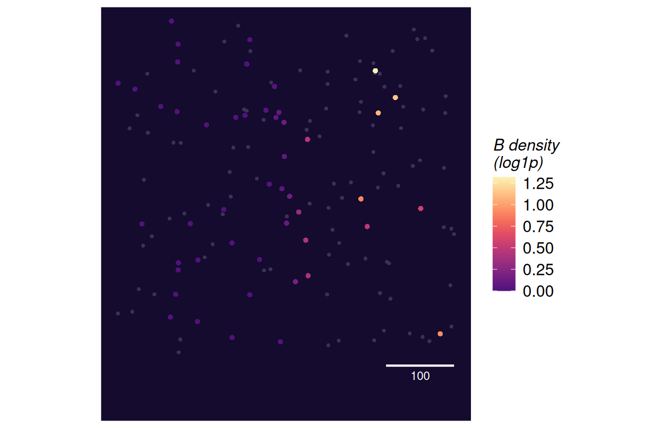
One sample’s cells, coloured by the log1p density of a niche type: the covariate spiDE regresses on. With index, only the index type’s cells are coloured – the covariate as the index type’s model reads it – and the others are dim. The panel is dark (the sticker’s ink) so that the lowest densities stay visible; the legend, titles and axes keep the page’s style.
plotNicheMap(
  spe,
  niche,
  sample,
  index = NULL,
  sigma = NULL,
  cell_type = "cell_type",
  sample_id = "sample_id",
  section = NULL,
  name = "Niche",
  point.size = NULL,
  scale.bar = TRUE,
  unit = NULL
)
spe
|
a SpatialExperiment with niche reducedDims (buildNiches()).
|
niche
|
a niche column (a cell type or a mergeNiches() group).
|
sample
|
the sample (patient) to show. |
index
|
NULL or an index cell type to highlight.
|
sigma
|
the bandwidth (needed only if spe carries several).
|
cell_type, sample_id
|
the colData columns of cell type and sample. |
section
|
NULL or the colData column of the section; a sample with several sections gets one panel each.
|
name
|
the niche reducedDim prefix. |
point.size
|
the point size (default: from the number of cells). |
scale.bar
|
draw a scale bar of about a fifth of the width. |
unit
|
the coordinates’ unit, for the scale bar’s label (e.g. “µm”).
|
Read it to judge the bandwidth: a speckled field that follows single cells is too small; a field nearly flat within a section is too large (the patient intercept then absorbs it). It also shows where the index cells sit relative to the niche.
a ggplot; p$data has one row per cell of the sample: x, y (from each section’s own origin), cell_type, density (log1p), section and focal (coloured).
library("spiDE")

data(toySpiDE)
spe <- buildNiches(toySpiDE, sigma = 30)
plotNicheMap(spe, niche = "B", sample = "S1", index = "A")