library("spiDE")
data(toySpiDE)
res <- spiDE(toySpiDE, condition = "condition", sigma = 30, verbose = FALSE)
plotCallMap(res, test = "pooled")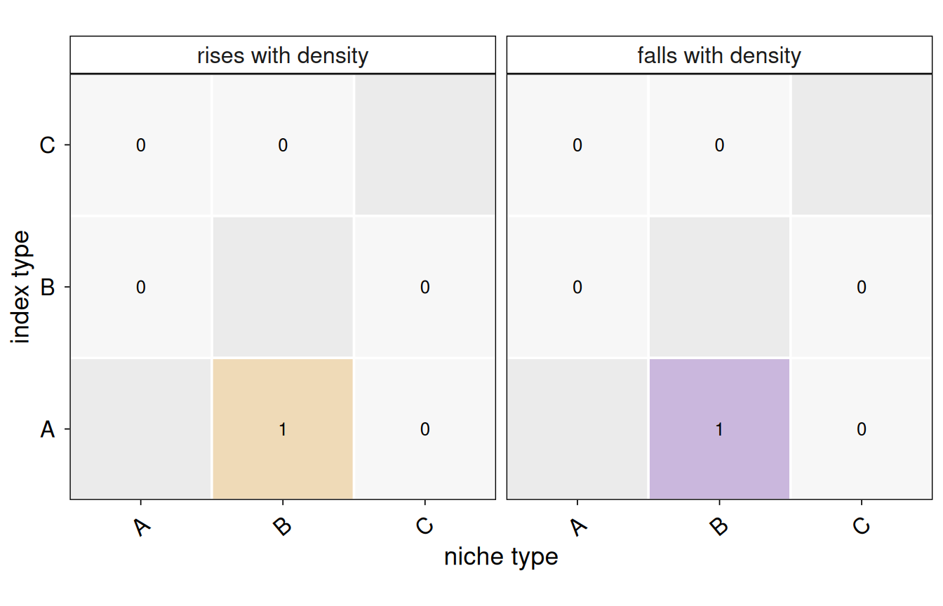
plotCallMap(res, style = "graph")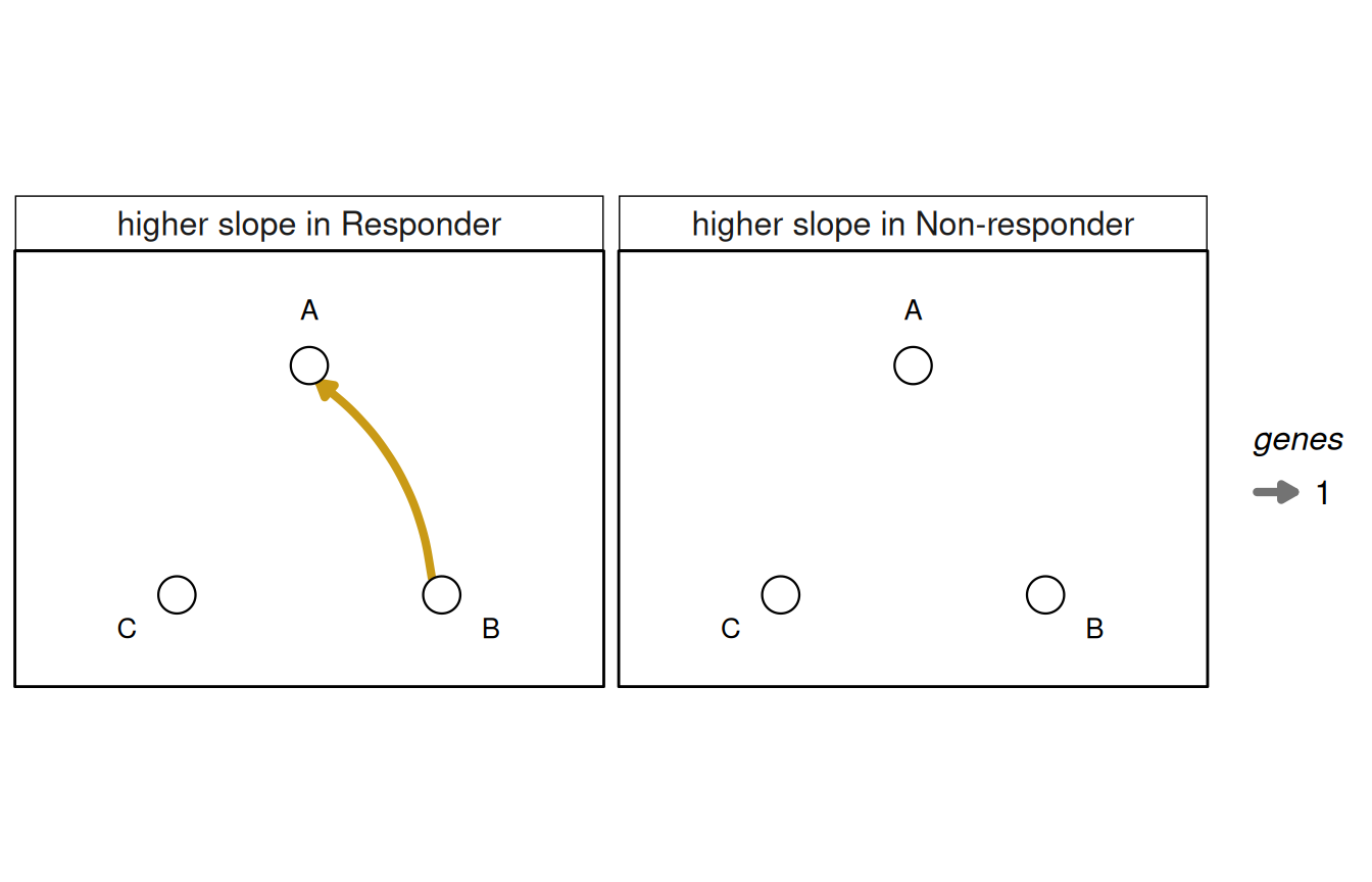
The number of genes called for every (index, niche) pair, split by direction: for the pooled test, a slope that rises or falls with the niche’s density; for the condition-specific test, a slope higher in one condition than in the other. The heatmap gives exact counts and marks untested pairs (an index type against its own niche) in grey; the graph draws cell types on a fixed circle with an arrow from niche to index type, its width the number of genes – it reads best when calls are few (the condition test), the heatmap when every pair has some.
plotCallMap(
  x,
  test = NULL,
  fdr = x@fdr,
  style = c("heatmap", "graph"),
  min.calls = 1L
)
x
|
a SpiDEResults. |
test
|
NULL (the condition-specific test if run, else the pooled test), “pooled” or “condition”.
|
fdr
|
the q-value threshold of a call. |
style
|
“heatmap” or “graph”.
|
min.calls
|
the graph’s smallest drawn edge. |
Read it for which cell-type pairs carry the signal, and for pairs whose calls all go one way toward one niche type (the shape segmentation spillover gives; see plotSpillover()). An arrow is an association, not signalling.
a ggplot. For the heatmap, p$data has one row per (index, niche, direction): calls and tested.
library("spiDE")

data(toySpiDE)
res <- spiDE(toySpiDE, condition = "condition", sigma = 30, verbose = FALSE)
plotCallMap(res, test = "pooled")
plotCallMap(res, style = "graph")