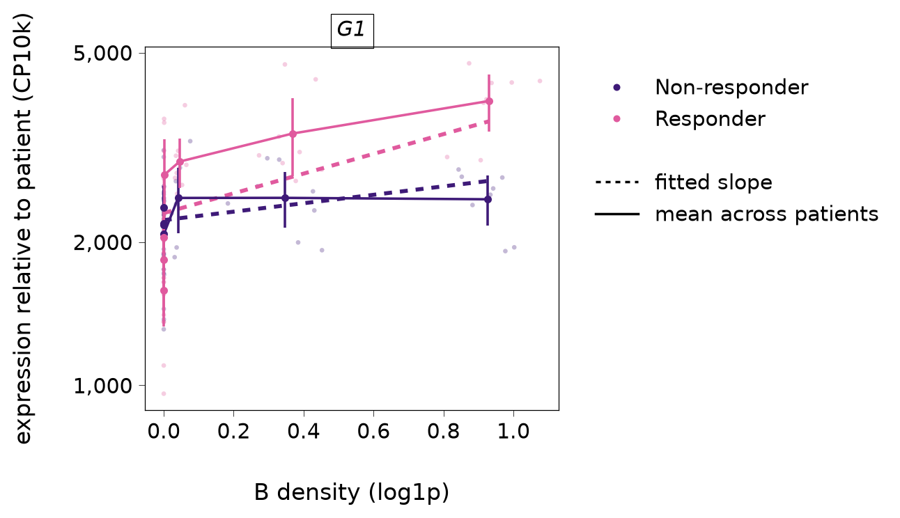
Expression against niche density: the cells behind a slope (R plotNicheResponse).
The index type’s cells’ expression of each gene (counts per 10,000, log axis) against the log1p density of the niche type, binned, one panel per gene.
With adjust=True (the default) each cell’s expression is divided by its patient’s fitted intercept, so the patients share one reference level and overlay: faint points are each patient’s mean in a density bin, points and bars the mean across patients and its 95% interval, per condition, and the dashed line each group’s fitted slope. This is what the tests compare. With adjust=False the data are raw: each patient’s own slope is a segment through its mean (open circle), and the dashed line through the patients’ means is the between-patient association that the intercepts absorb (test_niche_abundance’s question), not a niche slope.
Read it for the data behind a slope, whether the log1p scale is roughly linear, and whether a few extreme cells drive it. The display normalises depth by library size (the model fits a slope on it).
Parameters
Name
Type
Description
Default
adata
anndata.AnnData
The object the fit was made from.
required
res
SpiDEResults or SpiDEFit
adjust=True needs a fit that kept the patient intercepts. Under the sandwich engine every patient’s and group’s line has the pooled slope.
required
gene
str or sequence of str
One or more genes, one panel each.
required
index
str
The index cell type.
required
niche
str
The niche cell type.
required
adjust
bool
Divide out each patient’s intercept (see above).
True
bins
int
The number of density bins (adjust=True; bins are quantiles over all patients). Raw data use fifths of each patient’s own density range.
8
assay
str
The counts layer.
"counts"
name
str
The niche obsm prefix.
"Niche"
Returns
Name
Type
Description
matplotlib.figure.Figure
One panel per gene (a free log y axis each), with the condition and line legends.
See Also
plot_patient_slopes : The patients’ slopes behind a test. plot_niche_map : The niche density in tissue.